使用 matlab 的 surface 和 contour 画图

1 简介

matlab 提供了两个酷炫的函数surface 和contour 用来画多维函数的图形。通过这两个函数我们可以对多维函数进行更直观的观察。

本文以函数：

\begin{equation} \label{eq:1} z = x\exp(-x^{2} + y^{2}) \end{equation}

为例，介绍 surface 和 contour 的实用方法。

2 surface

看代码：

1: [X,Y] = meshgrid(-2:0.2:2,-2:0.2:2);
2: Z = X.*exp(-X.^2 - Y.^2);
3: figure
4: surface(X,Y,Z)
5: view(3)

结果如图：

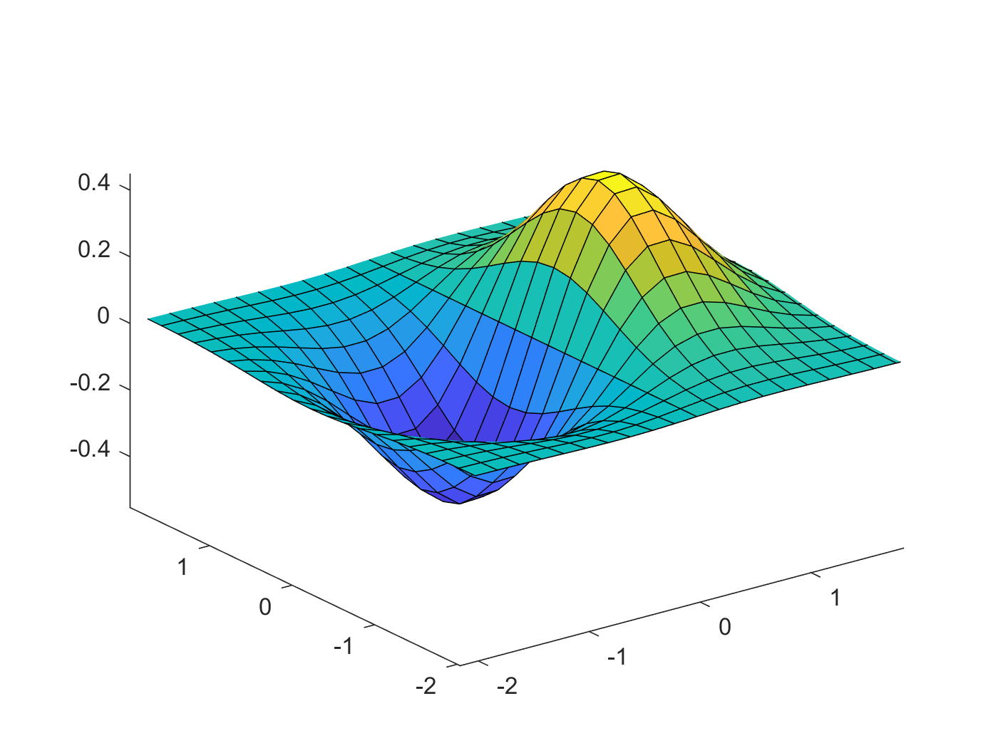
Figure 1: surface 示例

注意在画图的时候，最后一句 view(3) 是必须的。不然 matlab 会默认使用 view(2) ,看到的会是二维的平面截图。

3 contour

contour 的功能是画一个多维函数的等高线。

看代码：

1: x = -2:0.2:2;
2: y = -2:0.2:3;
3: [X,Y] = meshgrid(x,y);
4: Z = X.*exp(-X.^2-Y.^2);
5: 
6: figure
7: contour(X,Y,Z,'ShowText','on')

结果如图2：

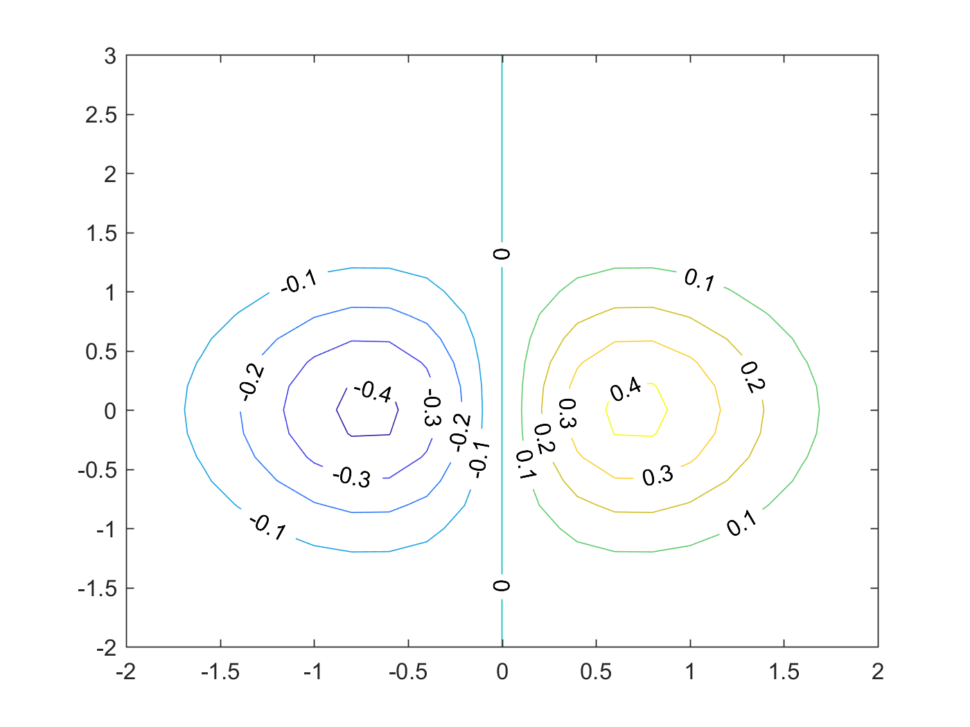
Figure 2: contour 示例

matlab 的帮助手册中有关于 contour 的更详细的说明，包括一些画图的技巧，等高线的间隔，高亮某条等高线等等。

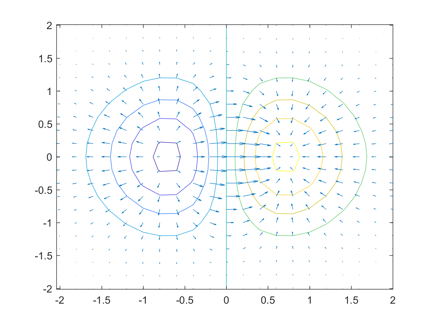
4 gradient

在 contour 的基础上，我们看看\(xe^{-x^{2} - y^{2}}\)的梯度示意图3。

1: x = -2:0.2:2;
2: y = x';
3: z = x .* exp(-x.^2 - y.^2);
4: [px,py] = gradient(z);
5: figure
6: contour(x,y,z)
7: hold on
8: quiver(x,y,px,py)
9: hold off

结果如图3所示：

Figure 3: \(xe^{-x^{2} - y^{2}}\)的梯度示意图

图3中的箭头所指是图1中从蓝色到橙色，即箭头部分永远指向更高的位置。

5 高维高斯分布

为了图形直观，以二维为例。向更高维度的扩展是显而易见的，但是通过contourf这样的函数实现高维几何直观就显得超出人类能力范围。

假设均值为\(\mathbf{\mu}\)，方差为\(\mathbf{\Sigma}\)，则高维高斯分布可以表示为：

\begin{equation} \label{eq:2} p(\mathbf{x}|\mathbf{\mu},\mathbf{\Sigma}) = \frac{1}{(2\pi)^{D/2} |\mathbf{\Sigma}|^{1/2} } \exp(- (\mathbf{x} - \mu)^{T}\mathbf{\Sigma}^{-1} (\mathbf{x} - \mathbf{\mu}) ) \end{equation}

 1: stepSize = 0.2; %0.05;
 2: [x,y] = meshgrid(-1:stepSize:1,-1:stepSize:1); % Create grid.
 3: [r,c]=size(x);
 4: data = [x(:) y(:)];
 5: p = func(data);
 6: p = reshape(p, r, c);
 7: 
 8: contourf(x,y,p,256,'LineColor','none');
 9: colormap(jet(256));
10: axis square;
11: set(gca,'XTick',[-1,0,1]);
12: set(gca,'YTick',[-1,0,1]);
13: xlabel(' W0 ');
14: ylabel(' W1 ','Rotation',0);
15:

这里的 func 是函数句柄。其原型为：

1: priorMean = [0;0];
2: priorSigma = eye(2)./priorPrecision; %Covariance Matrix
3: priorPDF = @(W)gaussProb(W,priorMean',priorSigma);

gaussProb 实现了式~(\ref{eq:2})。图4展示了最终的结果：

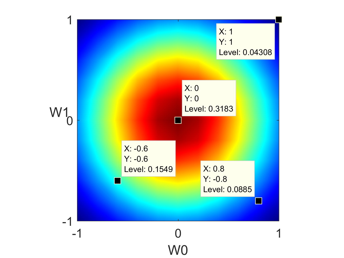
Figure 4: 使用countourf画二维高斯图形。

颜色越靠近红色，概率越高；越靠近蓝色概率越低。

当我们改变\(\mathbf{\mu}\)和\(\mathbf{\Sigma}\)的值时，其形状也会发生变化。比如，我们令:

\begin{equation} \label{eq:3} \mathbf{\mu} = [0.2 \quad 0.4] \end{equation} \begin{equation} \label{eq:4} \mathbf{\Sigma} = \begin{bmatrix} 0.4 & 0 \\ 0 & 0.2 \end{bmatrix} \end{equation}

其结果如图5所示：

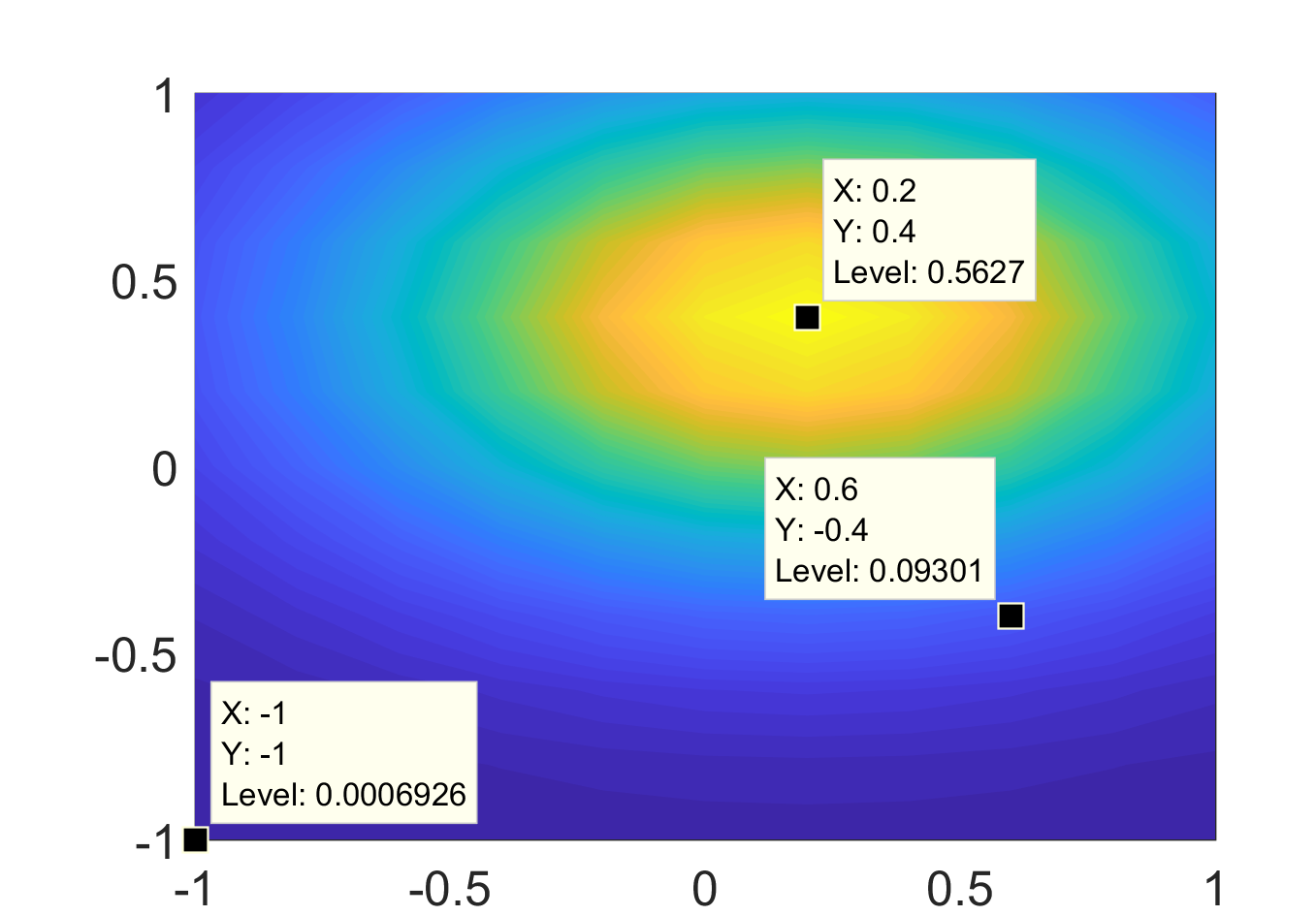
Figure 5: 使用countourf画二维高斯图形。

如果在上面的代码中使用 contour ，我们可以看到图6：

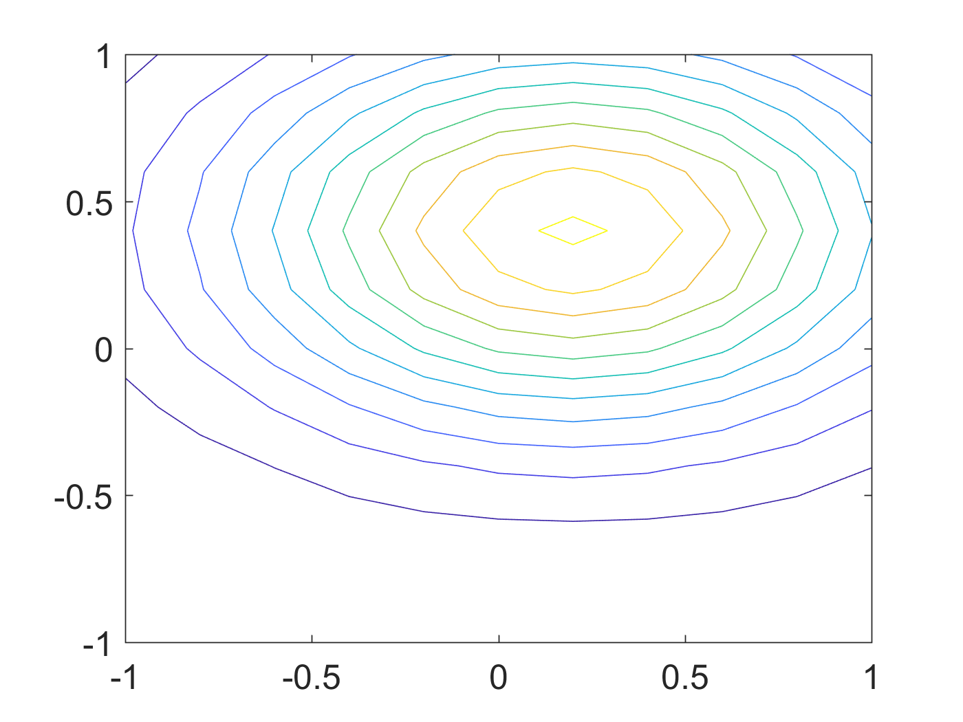
Figure 6: 使用countour画二维高斯图形。

contour 又找回了等高线的感觉， contourf 则为这些等高线之间进行颜色插值蒙上一个表面。